Tutorial¶

Fluxpart is a Python 3 module that implements the flux variance similarity method [SS08] for partitioning eddy covariance measurements of water vapor and carbon dioxide fluxes into stomatal (transpiration, photosynthesis) and nonstomatal (evaporation, respiration) components.

This tutorial assumes a basic familiarity with the Python programming language, the SciPy ecosystem, and the flux variance similarity partitioning procedure introduced by Scanlon and Sahu [SS08]. An overview of the flux partitioning algorithm is given in [SAAS+18] and here. Additional explanation of the partitioning method can be found in [SS08], [SK10], and [PRV14].

Notation and Definitions¶

The following notation is used in variable naming and documentation to represent meteorological quantities:

u, v, w = horizontal (u, v) and veritcal (w) wind velocities
q = water vapor mass concentration
c = carbon dioxide mass concentration
T = air temperature
P = total air pressure

The partitioning algorithm processes high-frequency eddy covariance data to determine interval average values for the water vapor and carbon dioxide fluxes:

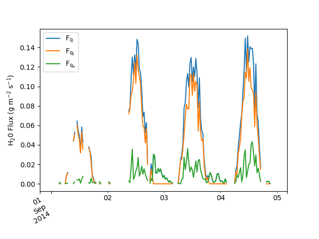
Fq = <w'q'> = Total H2O vapor flux
Fqe = <w'qe'> = Nonstomatal component of H2O vapor flux (evaporation)
Fqt = <w'qt'> = Stomatal component of vapor flux (transpiration)
Fc = <w'c'> = Total CO2 flux
Fcr = <w'cr'> = Nonstomatal component of CO2 flux (respiration)
Fcp = <w'cp'> = Stomatal component of CO2 flux (photosynthesis)

where a prime indicates the fluctuation of a scalar quantity and angle brackets indicate time averaging over an interval (e.g., 30 min).

The following definitions, relations, and requirements exist:

Fq = Fqe + Fqt
Fc = Fcr + Fcp
Fqe > 0
Fqt > 0
Fcr > 0
Fcp < 0
WUE = Fcp/Fqt < Fc/Fq < 0

where WUE is leaf-level water use efficiency.

Partitioning with `fvs_partition()`¶

A complete implementation of the flux variance similarity partitioning method is provided by the function fvs_partition().

The full procedure involves:

Reading high-frequency eddy covariance data
Performing basic data QA/QC
Making necessary data transformations (unit conversions, external effects corrections)
Estimating WUE if measurements are not available
Seeking a physically acceptable partitioning solution, progressively removing low frequency components from data as needed to conform with flux variance similarity assumptions

fvs_partition() has several parameters and options that specify how these procedures are performed. At a minimum, it is necessary to (i.) specify the location and format of high frequency data; and (ii.) provide either a value for the water use efficiency or other data needed to estimate water use efficiency.

Consider the following example. Suppose high frequency eddy covariance data for several years are stored as delimited text files in a directory /media/tower, each file holding 15 minutes of data with the file naming convention TOA5_YYYY_MM_DD_HHMM.dat.

Fluxes partitioned at 30 minute intervals for the dates May 1, 2014 through September 30, 2014 can be found found by:

from fluxpart import fvs_partition

data_files = "/media/tower/*_2014_0[4-9]_*"
results_file = "/media/results/apr-sept_2014.pkl"
heights_file = "/media/data/meta_heights.csv"
daylight_file = "/media/data/daylight2014.csv"

fvsp = fvs_partition(
    file_or_dir=data_files,
    hfd_format="EC-TOA5",
    interval="30min",
    wue_options={"heights": heights_file, "ppath": "C3"},
    part_options={"daytime": daylight_file},
)

fvsp.save(results_file)

Plotting a portion (Sept. 1–4) of the obtained water vapor mass fluxes:

import matplotlib.pyplot as plt
fig, ax = plt.subplots()
fvsp.plot_h2o(start="2014-09-01", end="2014-09-04", ax=ax)
fig.autofmt_xdate()
fig.savefig("/media/results/example_h2o.png")

Let’s consider individually the different parts of this example.

High frequency data location¶

The lines highlighted below specify the data location:

    from fluxpart import fvs_partition

    data_files = "/media/tower/*_2014_0[4-9]_*"
    results_file = "/media/results/apr-sept_2014.pkl"
    heights_file = "/media/data/meta_heights.csv"
    daylight_file = "/media/data/daylight2014.csv"

    fvsp = fvs_partition(
        file_or_dir=data_files,
        hfd_format="EC-TOA5",
        interval="30min",
        wue_options={"heights": heights_file, "ppath": "C3"},
        part_options={"daytime": daylight_file},
    )

    fvsp.save(results_file)

(Note that the file pathnames in this example are Unix-style. On Windows, the equivalent would be data_files = "C:/media/tower/*_2014_0[4-9]_*, etc.)

file_or_dir¶

file_or_dir is the pathname for the high frequency eddy covariance data file, data directory, or a list of either. Pathnames can be relative or absolute, and can include Unix shell-style wildcards (*, ?, and character ranges expressed with [ ]). If file_or_dir, or one or its elements, is a directory, then all files in that directory are read. For example:

file_or_dir="c:/some/path/file1.dat"
file_or_dir="../some/relpath/file*.tob"
file_or_dir="c:/some/path/*_201[12]_0[4-9]_*.dat"
file_or_dir=["c:/some/path/file1.tob", "C:/path/file2.tob"]
file_or_dir="/some/path"
file_or_dir=["../path1/*", "C:/path2/filename_??.dat"]

Related: Execution times and data files

High frequency data format¶

The highlighted line indicates the format of the high frequency data:

    from fluxpart import fvs_partition

    data_files = "/media/tower/*_2014_0[4-9]_*"
    results_file = "/media/results/apr-sept_2014.pkl"
    heights_file = "/media/data/meta_heights.csv"
    daylight_file = "/media/data/daylight2014.csv"

    fvsp = fvs_partition(
        file_or_dir=data_files,
        hfd_format="EC-TOA5",
        interval="30min",
        wue_options={"heights": heights_file, "ppath": "C3"},
        part_options={"daytime": daylight_file},
    )

    fvsp.save(results_file)

hfd_format¶

Normally, a dictionary of parameters specifying the file format is passed using the hfd_format argument. In this example, however, we take advantage of the fact that the file format matches one of the pre-defined data formats. So instead of a dictionary of format specifications, we simply pass a string indicating the name (“EC-TOA5”) of the pre-defined format. The equivalent dictionary specification for the “EC-TOA5” format is:

hfd_format = {
    "filetype": "csv",
    "cols": (2, 3, 4, 5, 6, 7, 8),
    "time_col": 0,
    "unit_convert": dict(q=1e-3, c=1e-6, P=1e3),
    "temper_unit": "C",
    "skiprows": 4,
    "na_values": "NAN",
    "to_datetime_kws": {"format": "ISO8601"},
}

When passing a custom hfd_format dictionary in this manner, it is required at a minimum to provide values for filetype and cols. time_col is also required if filetype is “csv”. unit_convert and temper_unit are required if data are not in SI units.

The primary hfd_format keys are:

hfd_format[“filetype”] : {“csv”, “tob1”, “ghg”, “pd.df”}, required: “csv” = delimited text file; “tob1” = Campbell Scientific binary data table format; “ghg” = LI-COR raw data format; “pd.df” = pandas dataframe.
hfd_format[“cols”] : 7*(int,), required: 7-tuple of integers indicating the data column numbers that contain series data for (u, v, w, c, q, T, P), in that order. Uses 0-based indexing.
hfd_format[“time_col”] : int, required for csv filetype: Datafile column containing datetime stamps. Uses 0-based indexing.
hfd_format[“unit_convert”] : dict: Dictionary of multiplication factors required to convert any u, v, w, c, q, or P data not in SI units to SI units (m/s, kg/m^3, Pa). (Note T is not in that list). The dictionary keys are the variable names. For example, if all data are in SI units except P and c, which are in kPa and mg/m^3, respectively, then set: hfd_options["unit_convert"] = {"P": 1e3, "c": 1e-6}, since it is necessary to multiply the kPa pressure data by 1e3 to obtain the SI pressure unit (Pa), and the mg/m^3 CO2 data by 1e-6 to obtain the SI concentration unit (kg/m^3). c and q data can be converted this way if they have units of mass or moles per volume. If instead the c and q data are given as mole fractions (e.g., mmol of q per mol dry air), then set the c and q converters to one of the following: “ppm_dry”, “ppt_dry”, “ppm_wet”, or “ppt_wet”. Use the “_dry” versions if the mole fraction data are w.r.t. to dry air (no water vapor) and “_wet” if they are w.r.t. moist air. For example, if q is in mmol q per mol dry air and c is umol c per mol dry air, then: {"P": 1e3, "q": "ppt_dry", "c": "ppm_dry"}.
hfd_format[“temper_unit”] : {“K”, “C”}: Temperature data units. Default is “K” (Kelvin).

When hfd_format[“filetype”] is “csv”, Fluxpart uses pandas.read_csv to read files. Any hfd_format key:value pairs not recognized by Fluxpart are passed to pandas.read_csv; See pandas.read_csv for an explanation of the many available formatting options, including “sep”, which permits reading text files delimited by characters other than “,”. The “EC-TOA5” definition uses two such keywords:

hfd_format[“skiprows”] : int: Number of header rows to skip at the top of the file.
hfd_format[“na_values”] :: String to be recognized as NaN, in addition the default list of NaN strings (see pandas.read_csv).
hfd_format[“to_datetime_kws”] :: Optional keyword arguments passed to pandas.to_datetime for reading datetimes.

A final hfd_format keyword recognized by Fluxpart, but not used in this example, is the “flags” key:

hfd_format[“flags”] : 2-tuple or list of 2-tuples: Specifies that one or more data columns are used to flag bad data records. Each tuple is of the form (col, goodval), where col is an int specifying the column number containing the flag (0-based indexing), and goodval is the value of the flag that indicates a good data record.

A second pre-defined format that is currently available uses the Campbell Scientific tob1 file format:

hfd_format="EC-TOB1"

which is equivalent to:

hfd_format = {
    "filetype": "tob1",
    "cols": (3, 4, 5, 6, 7, 8, 9),
    "temper_unit": "C",
    "unit_convert": dict(q=1e-3, c=1e-6, P=1e3),
}

With tob1 files, time_col is not used. The date and time are determined from the named “SECONDS” and “NANOSECONDS” columns.

A third pre-defined format uses the LI-COR raw data format:

hfd_format="EC-GHG1"

which is equivalent to:

hfd_format = {
    "filetype": "ghg",
    "sep": "\t",
    "cols": (11, 12, 13, 7, 8, 9, 10),
    "time_col": [5, 6],
    "unit_convert": dict(q=1e-3 * MW.vapor, c=1e-3 * MW.co2, P=1e3),
    "temper_unit": "C",
    "skiprows": 8,
    "na_values": "NAN",
    "to_datetime_kws": {"format": "%Y-%m-%d %H:%M:%S:%f"},
}

Water Use Efficiency¶

If the water use efficiency (WUE) is known, it is passed to fvs_partition() using the meas_wue argument. Note that according to the sign convention, WUE must be a negative value. meas_wue has units of kg CO2 / kg H2O. meas_wue can be a float value; the name of a delimited text file that has datetime stamps in the first column and wue values in the second; or a callable that takes a datetime object as its sole argument and returns a float value.

If WUE is not known, it must be estimated. The method and data used in the estimation are specified with wue_options.

wue_options¶

    from fluxpart import fvs_partition

    data_files = "/media/tower/*_2014_0[4-9]_*"
    results_file = "/media/results/apr-sept_2014.pkl"
    heights_file = "/media/data/meta_heights.csv"
    daylight_file = "/media/data/daylight2014.csv"

    fvsp = fvs_partition(
        file_or_dir=data_files,
        hfd_format="EC-TOA5",
        interval="30min",
        wue_options={"heights": heights_file, "ppath": "C3"},
        part_options={"daytime": daylight_file},
    )

    fvsp.save(results_file)

wue_options is a dictionary of parameters for specifying options related to estimating leaf-level water use efficiency (WUE) At a minimum, it is necessary to specify the photosynthetic pathway of the vegetation and the heights of the canopy and the eddy covariance instruments.

wue_options[“ppath”] : {“C3” or “C4”}: Photosynthetic pathway of the vegetation at the site

The heights can be specified in two ways, either separately as:

wue_options[“canopy_ht”] : float: Plant canopy height (meters)
wue_options[“meas_ht”] : float: Eddy covariance measurement height (meters)

or alternatively as:

wue_options[‘heights’]str or callable, optional: If str, is the name of a csv file with date strings in the first column, canopy heights in the second, and measurement heights in the third. If callable, accepts a date as its sole argument and returns the tuple of heights, (canopy_ht, meas_ht).

Example file of heights (header row optional):

date,canopy_height,tower_height
2012-04-05,4.27,6.61
2012-04-23,4.27,7.11
2012-05-07,4.42,7.11
...

When data are not given for a particular date, heights from the most recent (previous) available date are used.

Other (optional) wue_options are (see water_use_efficiency() for a full description of these options):

wue_options[“ci_mod”] : str: A string that indicates the model to be used to calculate the intercellular CO2 concentration (default is “const-ratio”).
wue_options[“ci_mod_param”] : float or 2-tuple of floats: Specific model parameter values to be used with the model indicated by wue_options["ci_mod"].
wue_options[“leaf_temper”] : float: The canopy leaf temperature (K) (set equal to the air temperature if not provided).
wue_options[“leaf_temper_corr”] : float: Adjustment applied to the (measured or estimated) canopy temperature (K) before calculating intercellular CO2. The temperature used in the intercellular CO2 calculation is leaf_T + wue_options["leaf_temper_corr"], where leaf_T is wue_options["leaf_temper"] if provided, and the air temperature otherwise. Default is wue_options["leaf_temper_corr"]=0.

Analysis Interval¶

    from fluxpart import fvs_partition

    data_files = "/media/tower/*_2014_0[4-9]_*"
    results_file = "/media/results/apr-sept_2014.pkl"
    heights_file = "/media/data/meta_heights.csv"
    daylight_file = "/media/data/daylight2014.csv"

    fvsp = fvs_partition(
        file_or_dir=data_files,
        hfd_format="EC-TOA5",
        interval="30min",
        wue_options={"heights": heights_file, "ppath": "C3"},
        part_options={"daytime": daylight_file},
    )

    fvsp.save(results_file)

When the time span of the high frequency data files does not match the desired time interval for data aggregation and flux partitioning, the data analysis interval is set with the interval argument. For example, the flux analysis interval is typically 15-60 min, whereas data may be stored in daily files. The time interval is specified using the pandas string alias format (e.g., interval="30min"). In the example above, the data were stored in 15 min files, but the analysis was done for 30 min data chunks. Setting interval to None treats whole, individual data files as the analysis interval (which is the default).

Partitioning Options¶

    from fluxpart import fvs_partition

    data_files = "/media/tower/*_2014_0[4-9]_*"
    results_file = "/media/results/apr-sept_2014.pkl"
    heights_file = "/media/data/meta_heights.csv"
    daylight_file = "/media/data/daylight2014.csv"

    fvsp = fvs_partition(
        file_or_dir=data_files,
        hfd_format="EC-TOA5",
        interval="30min",
        wue_options={"heights": heights_file, "ppath": "C3"},
        part_options={"daytime": daylight_file},
    )

    fvsp.save(results_file)

The part_options argument is a dictionary that can be used to set options for the partitioning algorithm. Currently, two fields are recognized:

part_options[“daytime”] : filename or callable or 2-tuple, optional: When specified, all fluxes for time intervals ending before sunrise or starting after sunset will be assumed non-stomatal. If a filename (str) is passed, the file is a csv file with date stamps in the first column, sunrise times in the second, and sunset in the third. If a callable is passed, the function should take a datetime.date object as its sole argument and return a 2-tuple of time objects. If a 2-tuple is passed, it is a tuple of python datetime.time objects for (sunrise, sunset).

Example daytime csv file:

date,sunrise,sunset
2014-01-01,07:10,16:54
2014-01-02,07:10,16:54
2014-01-03,07:10,16:55
...

When data are not given for a particular date, time from the most recent (previous) available date are used.

part_options[“adjust_fluxes”] : bool: If True (default), the final partitioned fluxes are adjusted proportionally such that sum of the partitioned fluxes match exactly the total fluxes indicated in the original data.

Additional Parameters and Options¶

Options for processing high frequency data¶

The hfd_options argument is a dictionary that can be used to set several optional parameters for processing the high frequency data. Note that several of these are activated by default.

hfd_options[“correct_external”] : bool, optional: If True (default), the water vapor and carbon dioxide series data are corrected for external fluctuations associated with air temperature and vapor density according to [WPL80] and [DK07].
hfd_options[“bounds”] : dict, optional: Dictionary indicating any lower and upper bounds for valid data. Dictionary entries have the form varname: (float, float), where varname is one of “u”, “v”, “w”, “q”, “c”, “T”, or “P”, and the 2-tuple holds values for the lower and upper bounds: (lower, upper). Data records are rejected if a variable in the record is outside the prescribed bounds. Default is bounds = {"c": (0, np.inf), "q": (0, np.inf)} such that data records are rejected if c or q data are not positive values.
hfd_options[“rd_tol”] : float, optional: Relative tolerance for rejecting the datafile. Default is hfd_options[“rd_tol”] = 0.4. See hfd_options[“ad_tol”] for further explanation.
hfd_options[“ad_tol”] : int, optional: Absolute tolerance for rejecting the datafile. Default is ad_tol = 1024. If the datafile contains bad records (not readable, out-of-bounds, or flagged data), the partitioning analysis is performed using the longest stretch of consecutive good data records found, unless that stretch is too short, in which case the analysis is aborted. The criteria for judging ‘too short” can be specified in both relative and absolute terms: the datafile is rejected if the good stretch is a fraction of the total data that is less than rd_tol, and/or is less than ad_tol records long.
hfd_options[“ustar_tol”] : float: If the friction velocity (m/s) determined from the high frequency data is less than ustar_tol, the partitioning analysis is aborted due to insufficient turbulence. Defalult is hfd_options[“ustar_tol”] = 0.1 (m/s).

Analysis and Visualization of Results¶

Perhaps the easiest way to get started working with results is to examine the examples in this Jupyter notebook. Additional detail is provided below.

`FluxpartResult`¶

fvs_partition() returns a FluxpartResult object. FluxpartResult is the composition of a datetime-indexed pandas DataFrame instance with a few convenience methods.

The columns in the DataFrame are multi-indexed. The top level labels are “fluxes”, “hfsummary”, “wue”, “fvsp_solution”, and “fluxpart”:

FluxpartResult.df.fluxes: The partitioned flux results.
FluxpartResult.df.hfsummary: Summary of the high frequency data.
FluxpartResult.df.wue: Summary of the water use efficiency estimation.
FluxpartResult.df.fvsp_solution: Computational details about the partitioning solution
FluxpartResult.df.fluxpart: Meta and summary information about the analysis

The DataFrame can be accessed via the df attribute, although it is usually not necessary since __getattr__ and __getitem__ passed to the DataFrame. For example, assuming the FluxpartResult has been named fvsp (as was done in the example above),

fvsp.fluxes

is the same as

fvsp.df.fluxes

Fluxpart results are stored in common units rather than SI units. For the fluxes, that means CO2 fluxes are in mg or umol per square meter per second, and that H2O fluxes are in g or mmol per square meter per second, or in W per square meter.

Because the output from fvs_partition() exists as a time-indexed pandas DataFrame, any number of data analyses and visualizations are possible. In addition to the notebook mentioned above, see the extensive pandas documentation for examples.

Saving and Opening Results¶

Saving results:

fvsp.save("my_results.pkl")

Opening saved results:

from fluxpart import fpread
fvsp = fpread("my_results.pkl")

Exporting Results¶

Since the results are stored as a DataFrame, the whole range of pandas export IO options are available.

For example, to export the entire multi-indexed DataFrame

fvsp.df.to_csv("export_fvsp_file.csv")

To export only the partitioned flux results,

fvsp.df.fluxes.to_csv("export_fvsp_fluxes.csv")